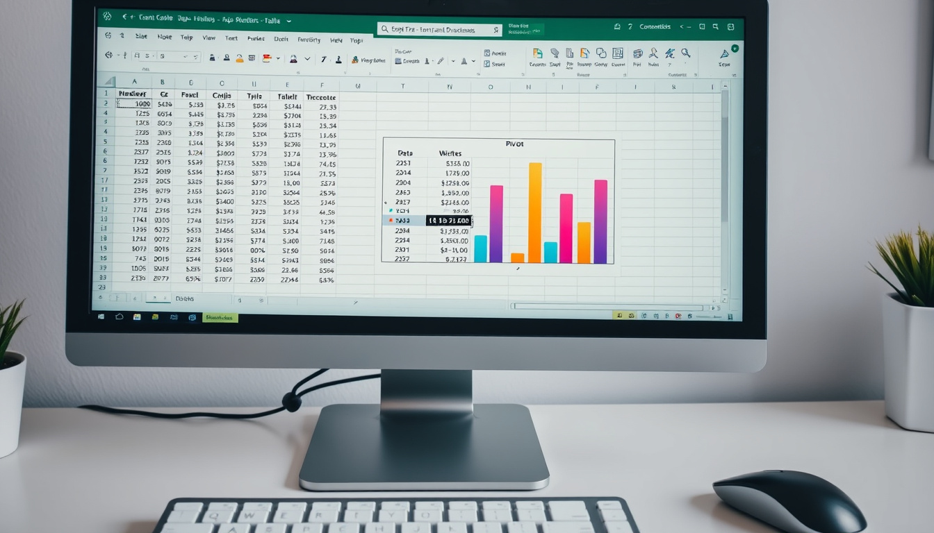
Anyone who’s stared at a spreadsheet full of rows and columns knows the feeling: there’s data in there, but getting it to tell a story takes work. That’s where Excel PivotTables come in—a tool that turns the grunt work of summarizing and analyzing into a few clicks.
Pivot table users worldwide: over 1 billion Excel users ·
Average time saved per report: 30 minutes ·
Data rows pivot tables can handle: 1,048,576 ·
Pivot table fields limit: 255 fields
Quick snapshot
- Click any cell in your data range (Excel Easy beginner guide)
- Go to Insert > PivotTable (Microsoft Support official documentation)
- Choose new or existing worksheet (GeeksforGeeks Excel tips)
- Drag fields to Rows, Columns, Values (DataCamp area explanation)
- Use Filters area for top-level slicers (Eval Academy guide)
- Reorder fields by dragging (Excel Guru workflow)
- Sum, count, average values automatically (Eval Academy analytics education)
- Change summary function via Value Field Settings (GeeksforGeeks Excel tips)
- Group dates by month, quarter, or year (Eval Academy analytics education)
- Use row/column label filters (Eval Academy filtering guide)
- Add slicers for quick filtering (Microsoft Support slicers documentation)
- Sort largest to smallest with one click (Eval Academy sorting guide)
The pattern across these steps: PivotTables give you flexibility without coding. Here’s what the official specs look like.
| Fact | Value |
|---|---|
| First introduced in Excel 97 | 1997 |
| Maximum rows in source data | 1,048,576 |
| Number of fields allowed per PivotTable | 255 |
| Available summary functions | Sum, Count, Average, Max, Min, Product, Count Numbers, StdDev, Var |
The implication: even with massive datasets, PivotTables stay within manageable limits—1,048,576 rows per source sheet and 255 fields is generous for most business reporting.
How to use PivotTable in Excel step by step?
Step 1: Prepare your data in a table format
- Start with a clean dataset: no blank rows or columns, a single header row, and one data type per column. Eval Academy data preparation guide emphasizes this as the most common beginner mistake.
- Highlight the entire dataset including column headers before moving to the Insert tab. GoSkills Excel tutorial recommends this to ensure no data is missed.
Step 2: Insert a PivotTable from the Insert tab
- Click any single cell inside your data range. Excel Easy beginner guide says this triggers Excel’s automatic range detection.
- Go to Insert > PivotTable. Microsoft Support official documentation confirms the Create PivotTable dialog box then appears with your selected range.
- Choose New Worksheet to keep your raw data separate—GeeksforGeeks Excel tips calls this the recommended approach for beginners.
Step 3: Drag fields into Rows, Columns, Values, and Filters areas
- In the PivotTable Fields pane, select the field name checkboxes to add them. Microsoft Support adding fields documentation describes this as the primary method.
- Drag a field to the Rows area to create row labels, to Columns for column headers, and to Values for calculations like sum or count. GeeksforGeeks area explanation breaks this down.
- For a first PivotTable, try Region in Rows, Quarter in Columns, and Revenue in Values—a classic example from Excel Guru beginner workflow.
Step 4: Refresh the PivotTable when source data changes
- Right-click anywhere inside the PivotTable and select Refresh to pick up new or changed data. Microsoft Support refresh documentation notes this is necessary because PivotTables don’t update automatically.
How do PivotTables work for beginners?
What is a PivotTable and how it summarizes data
- A PivotTable is a built-in Excel tool for summarizing, grouping, and analyzing large datasets interactively. Excel Guru definition puts it simply.
- Microsoft Support tool description defines it as a tool to analyze worksheet data by summarizing it interactively.
What are the four main areas: Rows, Columns, Values, Filters
- DataCamp Excel pivot areas guide identifies the four key areas: Filters, Columns, Rows, and Values.
- Rows create row labels, Columns create column headers, and Values add calculations like sum or count. GeeksforGeeks area roles explanation explains each.
How to drag and drop fields to rearrange the report
- Simply drag a field name from the field list to a different area, or reorder fields within an area. Excel Easy field rearrangement guide shows that dragging instantly updates the PivotTable layout.
New users often find the pivot table fields pane overwhelming, but the drag-and-drop approach means you can experiment without breaking anything—just pull fields around until the numbers tell your story.
The pattern: PivotTables replace ad-hoc formulas with a visual interface. You don’t write a SUMIF or COUNTIF—you check a box and the calculation happens.
What can I do with PivotTables in Excel?
Summarize sales data by product or region
- PivotTables let you aggregate thousands of rows into one summary table. Eval Academy aggregation example demonstrates how a single PivotTable can show total sales per region in seconds.
- Group data by product, category, region, or any text field. Eval Academy grouping guide shows date grouping by month, but the same logic applies to categories.
Compare monthly totals or year-over-year trends
- Drag a date field into Rows, then group by month or year. Eval Academy date grouping guide says Excel automatically creates hierarchical date groupings.
- To compare year over year, place years in Columns and months in Rows within the same PivotTable.
Filter data using slicers for interactive reports
- Slicers are visual filters that let users click buttons to show only certain data. Microsoft Support slicers documentation describes them as an intuitive filtering option added in Excel 2010.
- Timeline controls (available in Excel 2013 and later) filter date fields with a slider. Microsoft Support timeline documentation integrates them seamlessly with PivotTables.
Create pivot charts from PivotTable data
- Select any cell in the PivotTable, go to Insert > PivotChart, and choose a chart type. DataCamp pivot charts guide notes that pivot charts are dynamic—they update when the PivotTable changes.
PivotTables are fast for standard summaries, but they don’t support custom calculations like nested IF statements. For complex logic, combine a PivotTable with helper columns in the source data.
What this means: PivotTables let you switch between views—product vs region, month vs quarter—without rewriting formulas. That’s the real time-saver.
What are the basics of a pivot table?
Understanding the source data requirements
- Source data must be structured as a table with a clear header row and no blank rows or columns. Eval Academy data structure guide warns that blanks cause incorrect groupings.
- GeeksforGeeks data cleaning guide advises removing blank rows before creating a PivotTable.
How to choose fields for Row Labels, Column Labels, Values, and Report Filter
- Text and date fields typically go into Rows or Columns. Numeric fields go into Values. Excel Easy field placement guide recommends placing categorical data in Rows and numerical data in Values.
- Report Filters (Filters area) let you filter the entire PivotTable by one or more dimensions, like showing data for only a specific department. DataCamp report filters guide explains this.
How to sort and filter within a PivotTable
- Right-click a value in the PivotTable and choose Sort to reorder rows or columns. Eval Academy sorting guide shows one-click sorting from largest to smallest.
- Use the drop-down arrows on row or column labels to filter by text, date range, or values. Eval Academy filtering guide covers label and value filters.
How to create pivot table in Excel for different worksheets?
Using the PivotTable Wizard for multiple sheets
- For combining data from different sheets, use the PivotTable Wizard (press Alt+D+P to open it). DataCamp multiple sheets guide describes the wizard’s “Multiple consolidation ranges” option.
- The wizard expects each range to have matching column headers. Eval Academy data consistency guide stresses that columns must be identical across sheets.
Combining data from multiple worksheets into one PivotTable
- An alternative is to use Power Query (Get Data > From File > From Workbook) to merge tables before creating the PivotTable. Microsoft Support Power Query merge guide offers this as a more scalable approach for frequent updates.
- Once the data is merged into a single table, insert a PivotTable as usual. The advantage: you can refresh the connection when the source sheets change.
Consolidating ranges from different tables
- For one-off reports, the PivotTable Wizard’s “Consolidation” feature works without queries. GoSkills consolidation guide notes that it’s a quick fix but less flexible than Power Query.
The catch: the PivotTable Wizard is hidden in modern Excel ribbons. Power Query is the recommended path for consistent multi-sheet analysis.
Confirmed facts vs. What’s unclear
- PivotTables can be created from any data range or table (Microsoft Support official documentation)
- Excel limits PivotTables to 1,048,576 rows (Eval Academy analytics education)
- Fields in the Values area require numeric data to sum (GeeksforGeeks Excel tips)
- Whether all users find PivotTables easy to learn depends on data literacy (DataCamp guide)
- Some advanced grouping features may behave differently in newer Excel versions (Eval Academy analytics education)
“A PivotTable is designed to analyze worksheet data by summarizing it interactively.”
Microsoft Support official product documentation
“PivotTables are a built-in Excel tool for summarizing, grouping, and analyzing large datasets interactively.”
Excel Guru Excel training resource
“A common beginner recommendation is to place the PivotTable on a New Worksheet rather than the same sheet as the raw data.”
Microsoft Support best practice guide
“PivotTables can summarize data using sums, averages, and counts—all with no formulas.”
Eval Academy analytics education resource
If you’re working with personal budgets, you might also find our Best Apps for Budgeting 2026 guide useful—PivotTables can analyze spending patterns the same way. For tech productivity tips, check out our MAC address explainer for another angle on data organization.
The choice for beginners is simple: invest 20 minutes learning PivotTables, and you’ll save hours on every future report. Skip them, and you’re stuck writing manual formulas every time the boss asks for a regional breakdown.
youtube.com, youtube.com, youtube.com, youtube.com, youtube.com
Frequently asked questions
What are the advantages of using a PivotTable in Excel?
They save time by automatically summarizing thousands of rows, allow interactive rearranging of data, and work without formulas. According to DataCamp, the main advantage is speed—once you set one up, you can rotate dimensions in seconds.
How do I refresh a PivotTable after changing source data?
Right-click inside the PivotTable and select Refresh, or go to Data > Refresh All. Microsoft Support notes that PivotTables don’t update automatically, so you must refresh after any source data change.
Can I create a PivotChart from my PivotTable?
Yes. Select any cell in the PivotTable, then go to Insert > PivotChart. DataCamp explains that the chart updates dynamically when the PivotTable is refreshed.
How do I add a calculated field to a PivotTable?
In the PivotTable Fields pane, click the drop-down arrow next to the field list and choose “Add Calculated Field.” GeeksforGeeks provides a step-by-step for custom formulas like profit margin.
Why is my PivotTable showing blank cells and how do I fix it?
Blank cells usually mean the source data contains empty rows or columns. Eval Academy recommends filling blanks with a placeholder like “0” or removing the empty rows entirely.
What is the difference between a PivotTable and a regular table?
A regular table stores raw data, while a PivotTable summarizes that data interactively. Excel Guru notes that PivotTables are read-only for source data—you can’t edit the raw numbers inside a PivotTable.